5 Association tests

These exercises introduce association testing: how to find which genetic variants are associated with a phenotype.

5.1 Null model

The first step in an association test is to fit the null model. We will need an AnnotatedDataFrame with phenotypes. We have a sample annotation with a sample.id column matched to the GDS file, and a phenotype file with subject_id. (In this example, we use the 1000 Genomes IDs for both sample and subject ID.) For TOPMed data, it is also important to match by study, as subject IDs are not unique across studies.

# sample annotation
repo_path <- "https://github.com/UW-GAC/SISG_2019/raw/master"
if (!dir.exists("data")) dir.create("data")
sampfile <- "data/sample_annotation.RData"
if (!file.exists(sampfile)) download.file(file.path(repo_path, sampfile), sampfile)
annot <- TopmedPipeline::getobj(sampfile)
library(Biobase)
head(pData(annot))

##   sample.id subject.id Population          Population.Description sex
## 1   HG00096    HG00096        GBR British in England and Scotland   M
## 2   HG00097    HG00097        GBR British in England and Scotland   F
## 3   HG00099    HG00099        GBR British in England and Scotland   F
## 4   HG00100    HG00100        GBR British in England and Scotland   F
## 5   HG00101    HG00101        GBR British in England and Scotland   M
## 6   HG00102    HG00102        GBR British in England and Scotland   F
##   status
## 1      0
## 2      1
## 3      0
## 4      1
## 5      0
## 6      0

# phenotypes by subject ID
phenfile <- "data/phenotype_annotation.RData"
if (!file.exists(phenfile)) download.file(file.path(repo_path, phenfile), phenfile)
phen <- TopmedPipeline::getobj(phenfile)

# access the data with the pData() function
head(pData(phen))

##   subject_id sex age height   study
## 1    HG00096   M  47  165.3 study_1
## 2    HG00102   F  49  169.1 study_1
## 3    HG00112   M  46  167.9 study_1
## 4    HG00114   M  49  169.5 study_1
## 5    HG00115   M  35  161.1 study_1
## 6    HG00116   M  37  182.2 study_1

# access the metadata with the varMetadata() function
varMetadata(phen)

##                        labelDescription
## subject_id           subject identifier
## sex                       subject's sex
## age        age at measurement of height
## height           subject's height in cm
## study                  study identifier

# merge sample annotation with phenotypes
library(dplyr)
dat <- pData(annot) %>%
    left_join(pData(phen), by=c("subject.id"="subject_id", "sex"="sex"))
meta <- bind_rows(varMetadata(annot), varMetadata(phen)[3:5,,drop=FALSE])
annot <- AnnotatedDataFrame(dat, meta)
save(annot, file="data/sample_phenotype_annotation.RData")

We will test for an association between genotype and height, adjusting for sex, age, and study as covariates. If the sample set involves multiple distinct groups with different variances for the phenotype, we recommend allowing the model to use heterogeneous variance among groups with the parameter group.var. We saw in a previous exercise that the variance differs by study.

library(GENESIS)
nullmod <- fitNullModel(annot, outcome="height", covars=c("sex", "age", "study"), 
                        group.var="study", verbose=FALSE)
save(nullmod, file="data/null_model.RData")

We also recommend taking an inverse normal transform of the residuals and refitting the model. See the full procedure in the
pipeline documentation.

5.2 Single-variant tests

Now that we have a null model adjusting height for covariates, we can run an association test to look for genetic effects on height.

Single-variant tests are the same as in GWAS. We use the assocTestSingle function in GENESIS. First, we have to create a SeqVarData object including both the GDS file and the sample annotation containing phenotypes. We then create a SeqVarBlockIterator object to iterate over blocks of variants.

library(SeqVarTools)
gdsfile <- "data/1KG_phase3_subset_chr1.gds"
if (!file.exists(gdsfile)) download.file(file.path(repo_path, gdsfile), gdsfile)
gdsfmt::showfile.gds(closeall=TRUE) # make sure file is not already open
gds <- seqOpen(gdsfile)
seqData <- SeqVarData(gds, sampleData=annot)
iterator <- SeqVarBlockIterator(seqData, verbose=FALSE)
assoc <- assocTestSingle(iterator, nullmod)

## # of selected samples: 1,126

head(assoc)

##   variant.id chr     pos allele.index n.obs         freq      Score
## 1          1   1  970546            1  1126 0.0039964476 -0.1191236
## 2          2   1  985900            1  1126 0.0492895204 -1.6707553
## 3          3   1 1025045            1  1126 0.0004440497 -0.2795838
## 4          4   1 1265550            1  1126 0.0008880995 -0.1105487
## 5          5   1 1472676            1  1126 0.0071047957  0.3630992
## 6          6   1 1735725            1  1126 0.0022202487 -0.1300405
##    Score.SE Score.Stat  Score.pval
## 1 0.2577712 -0.4621292 0.643988703
## 2 0.8841849 -1.8895995 0.058811539
## 3 0.1007173 -2.7759261 0.005504472
## 4 0.1085480 -1.0184319 0.308472754
## 5 0.3456555  1.0504657 0.293504072
## 6 0.1973175 -0.6590420 0.509868791

We make a QQ plot to examine the results.

library(ggplot2)
qqPlot <- function(pval) {
    pval <- pval[!is.na(pval)]
    n <- length(pval)
    x <- 1:n
    dat <- data.frame(obs=sort(pval),
                      exp=x/n,
                      upper=qbeta(0.025, x, rev(x)),
                      lower=qbeta(0.975, x, rev(x)))
    
    ggplot(dat, aes(-log10(exp), -log10(obs))) +
        geom_line(aes(-log10(exp), -log10(upper)), color="gray") +
        geom_line(aes(-log10(exp), -log10(lower)), color="gray") +
        geom_point() +
        geom_abline(intercept=0, slope=1, color="red") +
        xlab(expression(paste(-log[10], "(expected P)"))) +
        ylab(expression(paste(-log[10], "(observed P)"))) +
        theme_bw()
}    

qqPlot(assoc$Score.pval)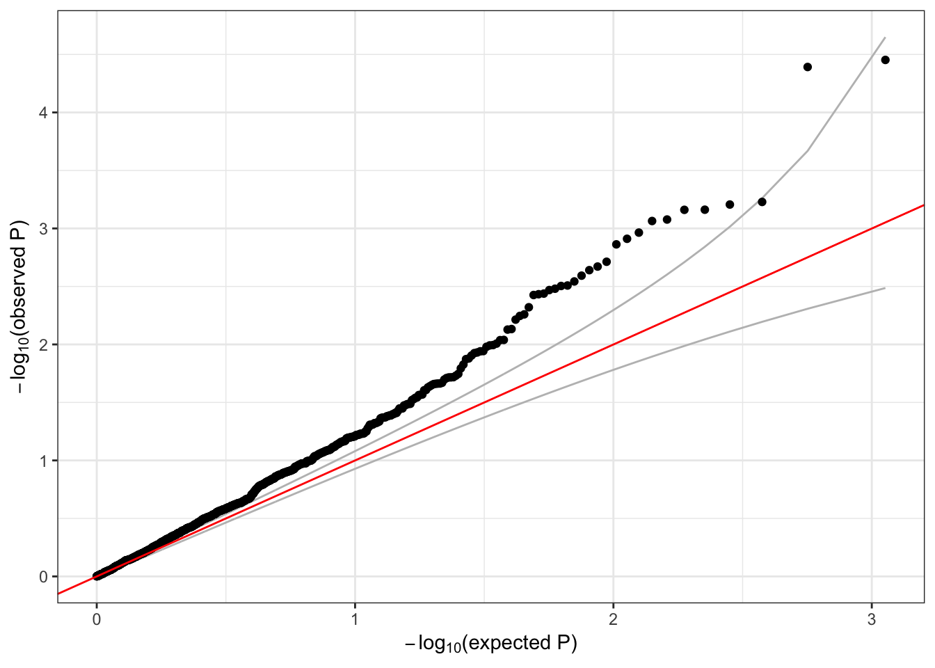

5.3 Exercises

Logistic regression: fitNullModel can use a binary phenotype as the outcome variable by specifying the argument family=binomial. Use the status column in the sample annotation to fit a null model for simulated case/control status, with sex and Population as covariates. Then run a single-variant test using this model.
Inverse normal transform: use the function nullModelInvNorm to perform an inverse normal transform on the height variable. Compare these residuals with the residuals from the original null model.

5.4 Sliding window tests

For rare variants, we can do burden tests or SKAT using the GENESIS function assocTestAggregate. We restrict the test to variants with alternate allele frequency < 0.1. (For real data, this threshold would be lower.) We use a flat weighting scheme. We define a sliding window across the genome using a SeqVarWindowIterator.

seqResetFilter(seqData, verbose=FALSE)
iterator <- SeqVarWindowIterator(seqData, windowSize=5000, windowShift=2000, verbose=FALSE)
assoc <- assocTestAggregate(iterator, nullmod, test="Burden", AF.max=0.1, weight.beta=c(1,1))

## # of selected samples: 1,126

names(assoc)

## [1] "results"     "variantInfo"

head(assoc$results)

##   chr   start     end n.site n.alt n.sample.alt      Score  Score.SE
## 1   1  966001  971000      1     9            9 -0.1191236 0.2577712
## 2   1  982001  987000      1   111          107 -1.6707553 0.8841849
## 3   1 1022001 1027000      1     1            1 -0.2795838 0.1007173
## 4   1 1262001 1267000      1     2            2 -0.1105487 0.1085480
## 5   1 1468001 1473000      1    16           16  0.3630992 0.3456555
## 6   1 1732001 1737000      1     5            5 -0.1300405 0.1973175
##   Score.Stat  Score.pval
## 1 -0.4621292 0.643988703
## 2 -1.8895995 0.058811539
## 3 -2.7759261 0.005504472
## 4 -1.0184319 0.308472754
## 5  1.0504657 0.293504072
## 6 -0.6590420 0.509868791

head(assoc$variantInfo)

## [[1]]
##   variant.id chr    pos allele.index n.obs        freq weight
## 1          1   1 970546            1  1126 0.003996448      1
## 
## [[2]]
##   variant.id chr    pos allele.index n.obs       freq weight
## 1          2   1 985900            1  1126 0.04928952      1
## 
## [[3]]
##   variant.id chr     pos allele.index n.obs         freq weight
## 1          3   1 1025045            1  1126 0.0004440497      1
## 
## [[4]]
##   variant.id chr     pos allele.index n.obs         freq weight
## 1          4   1 1265550            1  1126 0.0008880995      1
## 
## [[5]]
##   variant.id chr     pos allele.index n.obs        freq weight
## 1          5   1 1472676            1  1126 0.007104796      1
## 
## [[6]]
##   variant.id chr     pos allele.index n.obs        freq weight
## 1          6   1 1735725            1  1126 0.002220249      1

qqPlot(assoc$results$Score.pval)

For SKAT, we use the Wu weights.

seqResetFilter(seqData, verbose=FALSE)
iterator <- SeqVarWindowIterator(seqData, windowSize=5000, windowShift=2000, verbose=FALSE)
assoc <- assocTestAggregate(iterator, nullmod, test="SKAT", AF.max=0.1, weight.beta=c(1,25))

## # of selected samples: 1,126

head(assoc$results)

##   chr   start     end n.site n.alt n.sample.alt        Q_0      pval_0
## 1   1  966001  971000      1     9            9   7.318094 0.643988703
## 2   1  982001  987000      1   111          107 154.178280 0.058811539
## 3   1 1022001 1027000      1     1            1  47.823916 0.005504472
## 4   1 1262001 1267000      1     2            2   7.319239 0.308472754
## 5   1 1468001 1473000      1    16           16  58.518662 0.293504072
## 6   1 1732001 1737000      1     5            5   9.499539 0.509868791
##   err_0
## 1     0
## 2     0
## 3     0
## 4     0
## 5     0
## 6     0

head(assoc$variantInfo)

## [[1]]
##   variant.id chr    pos allele.index n.obs        freq   weight
## 1          1   1 970546            1  1126 0.003996448 22.70917
## 
## [[2]]
##   variant.id chr    pos allele.index n.obs       freq   weight
## 1          2   1 985900            1  1126 0.04928952 7.431881
## 
## [[3]]
##   variant.id chr     pos allele.index n.obs         freq   weight
## 1          3   1 1025045            1  1126 0.0004440497 24.73493
## 
## [[4]]
##   variant.id chr     pos allele.index n.obs         freq   weight
## 1          4   1 1265550            1  1126 0.0008880995 24.47255
## 
## [[5]]
##   variant.id chr     pos allele.index n.obs        freq   weight
## 1          5   1 1472676            1  1126 0.007104796 21.06793
## 
## [[6]]
##   variant.id chr     pos allele.index n.obs        freq   weight
## 1          6   1 1735725            1  1126 0.002220249 23.70132

qqPlot(assoc$results$pval)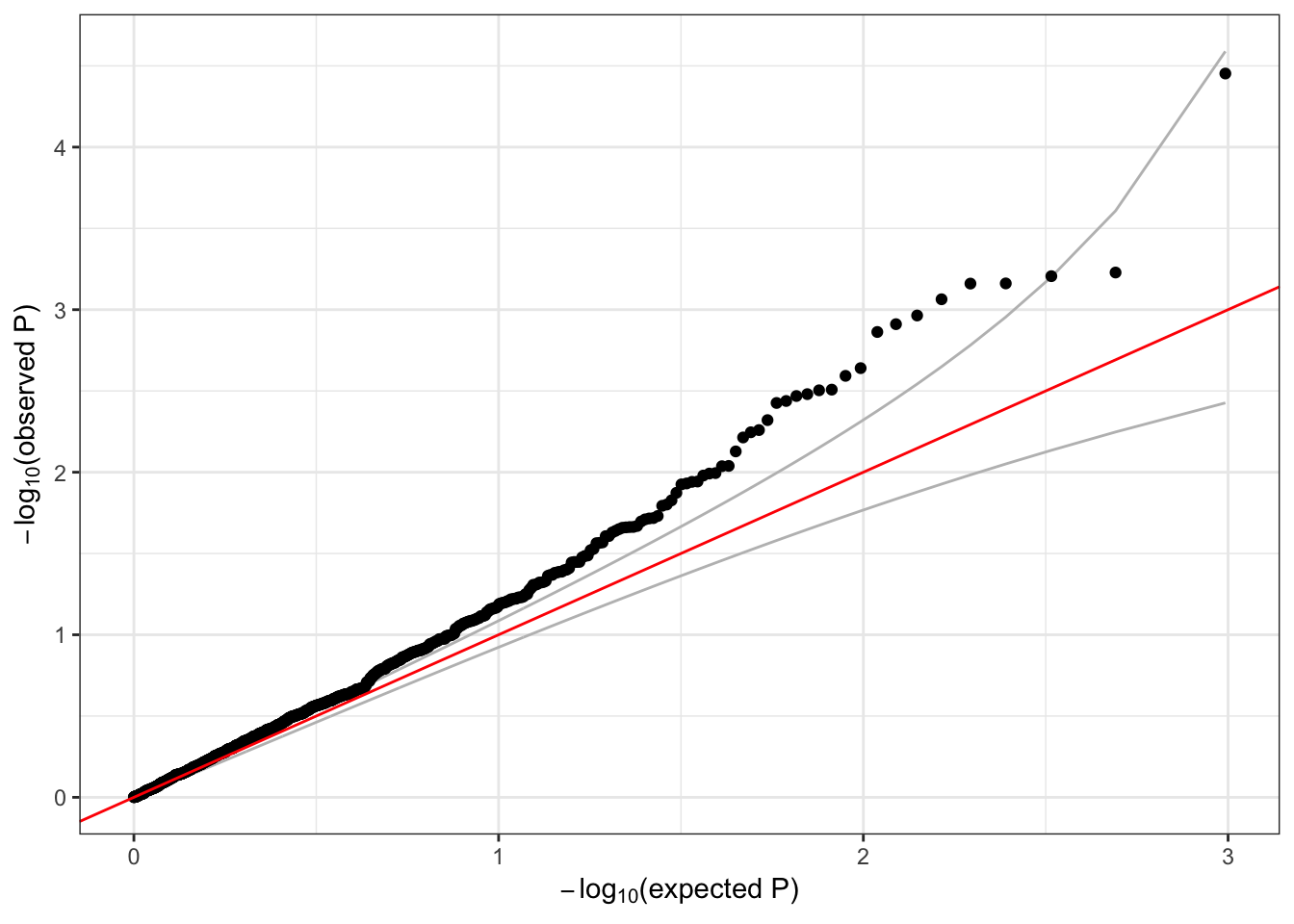

5.5 Exercise

Repeat the previous exercise on logistic regression, this time running a sliding-window test.